In the previous post we defined path integrals through a simple ‘time-slicing’ approach. And used them to compute moments of simple stochastic DEs. In this follow-up post we will examine how expansions can be used to approximate moments, how we can use the moment generating functional to compute probability densities, and how these methods may be helpful in some cases in neuroscience.

Perturbative approaches

For a general, non-linear, SDE the series will not terminate and must be truncated at some point. It is then necessary to determine which terms will contribute the sum, and to include these terms up to a given order. We mention briefly three such possibilities, though do not discuss them in any detail. One way of doing this is if some terms in $S_{I}$ ($v_{mn}\int x^{n}\tilde{x}^{m},m\ge2$) are small. Then we can simply let each such vertex contribute a small parameter $\alpha$ and perform an expansion in orders of $\alpha$ (known as a ‘weak coupling expansion’ ¹).

Another option is to perform a weak noise, or loop, expansion. Here we scale the entire exponent in the MGF by some factor $h$

Then each vertex of $S_{I}$ gains a factor of $1/h$ and each edge of $S_{F}$ gains a factor $h$ which implies we can expand in powers of $h$. In performing this expansion, if we let $E$ denote the number of external edges of a diagram, $I$ the number of internal edges and $V$ the number of vertices then each connected graph has a factor of \(h^{I+E-V}\) and, in fact, it can be shown by induction that: \(L=I-V+1\) where $L$ is the number of loops the diagram contains. Thus, each graph collects a factor of $h^{E-L+1}$. This allows us to order the expansion in terms of the number of loops in each diagram. Diagrams which contain no loops are trees, or classical diagrams. Such diagrams form the basis of the semi-classical approximation.

This expansion is of course only valid when the contribution of the higher loop number diagrams is smaller than that of the lower loop number diagrams. The Ginzburg criterion says when this expansion is indeed valid.

Some other examples

We present two further examples which demonstrate how these methods are used.

Example 1

A simple extension of the OU process so that it is now mean-reverting (to something not zero, as in the previous case) is the SDE

This problem is obviously very similar to the above problem and is of course solved almost identically. This time the action of the process is

such that the free action is as before:

(the linear, homogenous part, for which a Green’s function can be calculated) and the interacting action is:

The only details that change are thus that the vertex linear in $\tilde{x}(t)$ changes from

which adds an extra term to the expression for the mean:

Since only this internal vertex is affected, and the second order vertex ($D\tilde{x}(t)^{2}/2$) is unaffected, the solution for the second-order cumulant will in fact be the same as our original example:

Example 2

Consider the harmonic oscillator with noise:

where $\eta$ is a white noise process. Subject to initial conditions $x(0)=x_{0}$ and $\dot{x}(0)=v_{0}$ ($t_{0}=0$). The action for this process is

which we will split into free and interacting components:

The free action gives the propagator as the Green’s function:

which can be shown to be

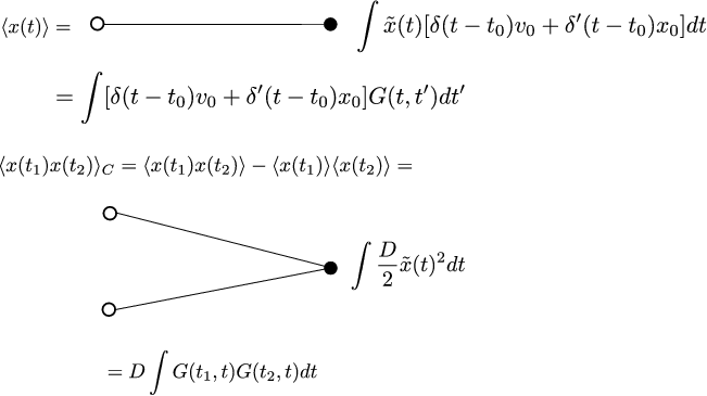
for $\omega_{1}=\sqrt{\omega^{2}-\gamma^{2}}$. Once $G$ is determined the mean and covariance can be immediately calculated through the diagrams and calculations of the Figure 1.

We find, as expected, the following mean and covariance:

and (assuming $t_{1}<t_{2}$)

which, with some rearrangement, simplifies to the variance²:

Connection to Fokker-Planck Equation

So far we have considered the moment generating functional, and the probability density functional $P[x(t)]$, however often of interest is the probability density $p(x,t)$. This can be computed from the above framework with the following derivation.

Let $U(x_{1},t_{1}|x_{0},t_{0})$ be the transition probability between a start point $x_{0},t_{0}$ to $x_{1},t_{1}$, then

where $Z_{CM}$ gives the moments of $x(t_{1})-x_{0}$ given $x(t_{0})=x_{0}$

Using the following two relations:

then $U$ becomes

From here we can derive a relation for $p(x,t)$:

and thus a PDE for $p(x,t)$:

as $\Delta t\to0$. This is the Kramers-Moyal expansion where the $D_{n}$ are

and are computed from the SDE. For example, for the Ito process

and $D_{2}(y,t)=g(y,t)^{2}$, $D_{n}=0$ for $n>2$. Hence the PDE becomes a Fokker-Planck equation

Compute $p(x,t)=U(x,t|0,0)$ as

For OU, we know the cumulants hence

Statistical mechanics of the neocortex

Having spent some time on how path integrals can be used as calculation devices for studying stochastic DEs, we now turn to some specific examples of their use in neuroscience.

Neural field models

A neural field model represents a continuum approximation to neural activity (particularly in models of cortex). They are often expressed as integro-differential equations:

where $U=U(x,t)$ may be either the mean firing rate or a measure of synaptic input at position $x$ and time $t$. The function $w(x,y)=w(|x-y|)$ is a weighting function often taken to represent the synaptic weight as a function of distance from $x$. $F(U)$ is a measure of the firing rate as a function of inputs. For tractability, $F$ may often be taken to be a heaviside function, or a sigmoid curve. It is called a field because each continuous point $x$ is assigned a value $U$, instead of modelling the activity of individual neurons. A number of spatio-temporal pattern forming systems may be studied in the context of these models. The formation of ocular-dominance columns, geometric hallucinations, persistent ‘bump models’ of activity associated with working memory, and perceptual switching in optical illusions are all examples of pattern formation that can be modelled by such a theory. Refer to Bressloff 2012 for a comprehensive review.

The addition of additive noise to the above model:

for $dW(x,t)$ a white noise process has been studied by Bressloff from both a path integral approach, and by studying a perturbation expansion of the resulting master equation more directly. We describe briefly how the path integral approach is formulated, and the results that can be computed as a result. More details are found in Bressloff 2009.

As above, this is discretized in both time and space to give:

for initial condition function $\Phi(x)=U(x,0).$ Where each noise process is a zero-mean, delta correlated process:

Let $U$ and $W$ represent vectors with components $U_{i,m}$ and $W_{i,m}$ such that we can write down the probability density function conditioned on a particular realization of $W$:

where we again use the Fourier representation of the delta function:

Knowing the density for the random vector $W$ we can write the probability of a vector $U$:

Taking the continuum limit gives the density:

for action

Given the action, the moment generating functional and propagator can be defined as previously. In linear cases the moments can be computed exactly.

The weak-noise expansion

If the noise term is scaled by a small parameter, $g(U)\to\sigma g(U)$ for $\sigma\ll1.$ (For instance, in the case of a Langevin approximation to the master equation, it is the case that $\sigma\approx1/N$ for $N$ the number of neurons.) Rescaling variables $\tilde{U}\to\tilde{U}/\sigma^{2}$ and $\tilde{J}\to\tilde{J}/\sigma^{2}$ then the generating functional becomes:

which can be thought of in terms of a loop expansion described above. Performing the expansion in orders of $\sigma$ allows for a ‘semi-classical’ expansion to be performed. The corrections to the deterministic equations take the form

for $C(x,y,t)$ the second-order cumulant (covariance) function. The expression for $C(x,y,t)$ is derived and studied in more detail in Buice et al 2010.

Mean-field Wilson-Cowan equations and corrections

Another approach using path integrals has been extensively studied by Buice and Cowan (Buice2007, see also Bresslof 2009). Here, we envision a network of neurons which exist in one of either two or three states, depending on the time scales of interest relative to the time scales of the neurons being studied. Each neuron in the network is modeled as a Markov process which transitions between active and quiescent states (and refractory, if it’s relevant).

For the two state model, assume that each neuron in the network creates spikes and that these spikes have an impact on the network dynamics for an exponentially distributed time given by a decay rate $\alpha.$ Let $n_{i}$ denote the number of ‘active’ spikes at a given time for neuron $i$ and let $\mathbf{n}$ denote the state of all neurons at a given time. We assume that the effect of neuron $j$ on neuron $i$ is given by the function

for some firing rate function $f$ and some external input $I$. Then the master equation for the state of the system is:

where we denote by \(\mathbf{n}_{i\pm}\) the state of the network \(\mathbf{n}\) with one more or less active spike in neuron $i$. The assumption is made that each neuron is identical and that the weight function \(w_{ij}=w_{|i-j|}\), that is, it only depends on the distance between the two neurons. Of interest is the mean activity of neuron $i$:

Using an operator representation it is possible to derive a stochastic field theory in the continuum limit ($N\to\infty$ and $n_{i}(t)\to n(x,t)$) to give moments of $n_{i}(t)$ in terms of the the interaction between two fields $\varphi(x,t)$ and $\tilde{\varphi}(x,t)$. The details of the derivation are contained in the Appendices of Buice and Cowan 2007. These fields can be related to quantities of interest through

and

for $t_{1}>t_{2}$. The propagator, as before, is

and the generating function is given by

For the master equation above the action is given by:

for convolution $\star$ and initial condition vector $\bar{n}(x).$ This now allows the action to be divided into a free and interacting action and for perturbation expansions to be performed.

The loop expansion provides a useful expansion and, as described in Section 2, amounts to ordering Feynman diagrams by the number of loops contained in them. The zeroth order, mean field theory, corresponds to Feyman diagrams containing zero loops. Such diagrams are called tree diagrams. It can be shown that the dynamics of this expansion obey: \(\partial_{t}a_{0}(x,t)+\alpha a_{0}(x,t)-f(w\star a_{0}(x,t)+I)=0\) which are also a simple form of the well known Wilson-Cowan equations. That these equations are recovered as the zeroth order expansion of the continuum limit of the master equation gives confidence that the higher-order terms of the expansion will indeed correspond to relevant dynamics. The ‘one-loop’ correction is given by:

for

and the ‘tree-level’ propagator

Summary

We have described how path integrals can be used to compute moments and densities of a stochastic differential equation, and how they can be used to perform perturbation expansions around ‘mean-field’, or classical, solutions.

Path integral methods, once one is accustomed to their use, can provide a quick and intuitive way of solving particular problems. However, it is worth highlighting that there are few examples of problems which can be solved with path integral methods but not with other, perhaps more standard, methods. Thus, while they are a powerful and general tool, their utility is often countered by the fact that, for many problems, simpler solution techniques exist.

Further, it should be highlighted that the path integral as it was defined here – as a limit of finite-dimensional integration ($\int\prod_{i}^{N}dx_{i}\to\int\mathcal{D}x(t)$) – does not result in a valid measure. In some cases the Weiner measure may equivalently be used, but in other cases the path integral as formulated by Feynman remains a mathematically unjustified entity.

With these caveats in mind, their principle benefit, then, may instead come from the intuition that they bring to novel mathematical and physical problems. When unsure how to proceed, having as many different ways of approaching a problem can only be beneficial. Indeed, in 1965 Feynman said in his Nobel acceptance lecture: “Theories of the known, which are described by different physical ideas may be equivalent in all their predictions and are hence scientifically indistinguishable. However, they are not psychologically identical when trying to move from that base into the unknown. For different views suggest different kinds of modifications which might be made and hence are not equivalent in the hypotheses one generates from them in one’s attempt to understand what is not yet understood.”