Path integrals and SDEs in neuroscience

An introduction to the relation between path integrals and stochastic differential equations, and how to use Feynman diagrams.

Introduction

The path integral was first considered by Wiener in the 1930s in his study of diffusion and Brownian motion. It was later co-opted by Dirac and by Richard Feynman in Lagrangian formulations of quantum mechanics. They provide a quite general and powerful approach to tackling problems not just in quantum field theory but in stochastic differential equations more generally. There is an associated learning curve to being able to make use of path integral methods, however, and for many problems simpler solution techniques exist.

Nonetheless, it is interesting to think about their application to neuroscience. In the following two posts I will describe how path integrals can be defined and used to solve simple SDEs, and why such ‘statistical mechanics’ tools may be useful in studying the brain. The following largely follows material from the paper “Path Integral Methods for Stochastic Differential Equations”, by Carson Chow and Michael Buice, 2012. This post will assume some familiarity with probability and stochastic processes.

Statistical mechanics in the brain

The cerebral cortex is the outer-most layer of the mammalian brain. In a human brain the *neocortex *consists of approximately 30 billion neurons. Of all parts of the human brain, its neural actvity is the most correlated with our *high-order *behaviour: language, self-control, learning, attention, memory, planning. Lesion and stroke studies make clear that the cortex has signficant functional localization, however, despite this localization, individual neurons from different regions of cortex in general require expert training to distinguish – these differences in functionality appear to arise largely from differences in connectivity.

The interplay between structural homogeniety and functional heterogeneity of different cortical regions poses definitive challenges to obtaining quantitative models of the large-scale activity of the cortex. Since structured neural activity is observed on spatial scales involving thousands to billions of neurons, and given that this activity is associated with particular functions and pathologies, dynamical models of large-scale cortical networks are definitely necessary to an understanding of these functions and dysfunctions. Examples of large-scale activities include wave-like activity during development, bump models of working memory, avalanches in awake and sleeping states, and pathological oscillations responsible for epileptic seizure.

A particular challenge to building such models is noise: it is well known that significant neural variability at both the individual and population level exists in response to repeated stimuli. The spike trains of individual cortical neurons are in general very noisy, such that their firing is often well approximated by a Poisson process. The primary source of cell intrinsic noise is fluctuations in ion channel activity, which arises from a finite number of ion channels opening and closing. While the primary source of extrinsic noise is from uncorrelated synaptic inputs – a neuron may contain thousands of synapses whose inputs often do not contain meaningful, correlated input. Population responses similarly exhibit highly variable responses. Models of cortical networks must account for this variability, or demonstrate that it is irrelevant to the particular questions being asked.

Methods from statistical mechanics lend themselves well to modelling both of these factors – statistical, but meaningful, connectivity, and noisy, but meaningful, neural responses to stimulus – in networks with large numbers of neurons. With these thoughts in mind, let’s see how path integrals may be used to study SDEs relevant to tackling the above issues.

A path integral representation of stochastic differential equations

We will begin by describing in some detail how they are constructed and manipulated. In general, we would like to study SDEs that may be of the form:

for some noise process $\eta(t).$ Such a process may be characterized by either its probability density function (pdf, $p(x,t)$) or, equivalently, by its moment heirarchy

A generic SDE in the above form may be studied as either a Langevin equation, or can be written as a Fokker-Planck equation, but perturbation methods in either of these forms may be difficult to apply. The path integral approach is able to provide more mechanical methods for performing particular types of perturbation expansions. In the following sections we will derive a path integral formulation of a moment generating funcational of an SDE, using the Ornstein-Uhlenbeck process as an example. This will be used to demonstrate the use of perturbation techinques using Feynman diagrams. We will also derive the pdf $p(x,t)$ of such a process.

Path integrals

A path integral, loosely, is an integral in which the domain of integration is not a subset of a finite dimensional space (say $\mathbb{R}^{n}$) but instead an infinite dimensional function space. For instance, if we can define the probability density associated with a particular realization of a random trajectory according to a given SDE, then the probability that a particle travels from a point $\mathbf{a}$ to a point $\mathbf{b}$ can be computed by marginalizing (summing) over all paths connecting these two points, subject to a suitable normalization. Before taking this further it is useful to review some relevant concepts.

Moment generating functions

The moment generating function (MGF) forms a crucial component to this framework. Recall that for a single random variable $X$, the moments ($\langle X\rangle=\int x^{n}P(x)\, dx$) are obtained from the MGF

by taking derivatives

and that the MGF contains all information about RV $X$, as an alternative to studying the pdf directly.

In a similar fashion we can define \(W(\lambda)=\log Z(\lambda),\) so that

are the cumulants of RV $X$.

For an $n$-dimensional random variable $\mathbf{x}=(x_{1},\dots,x_{n})$, the generating function is

for $\lambda=(\lambda_{1},\dots,\lambda_{n})$. Here, the $k$-th order moments are obtained via

And, as before, the cumulant generating function is $W(\lambda)=\log Z(\lambda)$.

Stochastic processes

Instead of considering random variables in $n$ dimensions, we can consider ‘infinite dimensional’ random variables through a time-slicing limiting process. That is, we identify with each $x_{i}$ in $\mathbf{x}$ a time $t=ih$ such that $x_{i}=x(ih)$, and we let total time $T=nh$, thereby splitting the interval $[0,T]$ into $n$ segments of length $h.$ From here, leaving any questions of convergence, etc, aside for the time being, we can take the limit $n\to\infty$ (with $h=T/n$) such that $x_{i}\to x(ih)=x(t)$, $\lambda_{i}\to\lambda(t)$ and $P(\mathbf{x})\to P[x(t)]=\exp(-S[x(t)])$ for some functional $S[x]$ that we will call the action. Thus we envision that to compute the MGF, instead of summing over all points in $\mathbb{R}^{n}$ $\left(\int\prod_{i=1}^{n}dx_{i}\right)$, we are instead summing over all paths using a differential denoted $\int\mathcal{D}x(t)$:

From this formula, moments can now be obtained via

with the cumulant generating functional again being

Generic Gaussian processes

The most important random process we consider is the Gaussian. Recall that in one dimension the RV $X\sim N(a,\sigma^{2})$ has MGF

which is obtained by a ‘completing the square’ manipulation, and has cumulant GF

so that the cumulants are $\langle x\rangle_{C}=a,\langle x^{2}\rangle_{C}=\text{var}{X}=\sigma^{2}$ and $\langle x^{k}\rangle_{C}=0$ for all $k>2$.

The $n$ dimensional Gaussian RV $X\sim N(0,K)$, with covariance matrix $K$, has MGF

This integral can also be integrated exactly. Indeed, since $K$ is symmetric positive definite (and so is $K^{-1}$), we can diagonalise in orthonormal coordinates, making each dimension independent, and allowing the integration to be performed one dimension at a time. This provides $Z(\lambda)=[2\pi\det(K)]^{n/2}e^{\frac{1}{2}\sum_{jk}\lambda_{j}K_{jk}\lambda_{k}}.$ In an analogous fashion, through the same limiting process described above, the infinite dimensional case is

Importantly for perturbation techniques, higher order (centered) moments of multivariate Gaussian random variables can be expressed simply as a sum of products of their second moments. This result is known as Wick’s theorem:

for $A={\text{all pairings of }x_{(i)}}$. Only even moments are non-zero. Note that this means that the covariance matrix $K$ is the key to determining all higher order moments. Wick’s theorem lies at the heart of calculations utilizing Feynman diagrams.

Applications to SDEs

The previous construction for generic Gaussian processes can be adapted to construct a moment generating functional for generic SDEs of the form

for $t\in[0,T]$. The process involves the same time-slicing approach, in which the above SDE is discretized in time steps $h$

under the Ito interpretation. We assume that each $w_{i}$ is a Guassian with $\langle w_{i}\rangle=0$ and $\langle w_{i}w_{j}\rangle=\delta_{ij}$ such that $w_{i}$ describes a Guassian white noise process. Then the PDF of $\mathbf{x}$ given a particuar instantiation of a random walk ${w_{i}}$ is

If we take the Fourier transform of the PDF:

where we’ve made use of the fact that the Dirac delta function has Fourier transform:

Marginalizing over all random trajectories ${w}$ and evaluating the resulting Gaussian integral gives:

Again we take the continuum limit by letting $h\to0$ with $N=T/h$, and by replacing $ik_{j}$ with $\tilde{x}(t)$ and ${\displaystyle \frac{x_{j+1}-x_{j}}{h}}$ with $\dot{x}(t)$:

The function $\tilde{x}(t)$ represents a function of the wave numbers $k_{j}$, thus we can write down a moment generating functional for both its position and its conjugate space:

More generally, instead of $g(x)\eta(t)$ with $\eta(t)$ a white noise process, an SDE having a noise process with cumulant $W[\lambda(t)]$ will have the PDF:

If $\eta(t)$ is delta correlated ($\langle\eta(t)\eta(t’)\rangle=\delta(t-t’)$) then $W[\tilde{x}(t)]$ can be Taylor expanded in both $x(t)$ and $\tilde{x}(t)$:

Note that the summation over $n$ starts at one because $W[0]=\log(Z[0])=0$.

The Ornstein-Uhlenbeck process

As an example, consider the Orstein-Uhlenbeck process

which has the action

The moments could found immedately, since action is quadratic in $\tilde{x}(t)$[^1], however we instead demonstrate how to study the problem through a perturbation expansion. In this case the perturbation will truncate to the exact, and already known, solution. The idea is to break the action into a ‘free’ and ‘interacting’ component. The terminology comes from quantum field theory in which free terms typically represent a particle without any interaction with a field or potential, and would have a quadratic action. The free action can therefore be evaluated exactly, and the interaction term can be expressed as an ‘asymptotic series’ around this solution. Let the action be written

We define the function $G$, known as the the linear response function or correlator or propagator, to be the Green’s function of the linear differential operator corresponding to the free action:

Note that $G(t,t’)$ is in fact exactly equivalent to $K(t,t’)$ from the generic Gaussian stochastic process derived previously. Note also that, in general, the ‘inverse’ of a Green’s function$G(t,t’)$ is an integral operator satisfying:

for some $G^{-1}(t,t’)$. The operator $\mathcal{L}$ would indeed be such an inverse for the following choice of $G^{-1}$:

The free generating functional, then, is

So, analogous to the multivariate Gaussian case, we can evaluate this integral exactly to obtain:

For the OU process we can in fact solve the linear differential equation for Green’s function $G$: \(G(t,t')=H(t-t')e^{-a(t-t')}.\) The free moments are then given by

Importantly, note that

and $\langle\tilde{x}(t_{1})\tilde{x}(t_{2})\rangle_{F}=\langle x(t_{1})x(t_{2})\rangle_{F}=0$.

Since the only non-zero second order moments are those in which an $x(t)$ is paired with an $\tilde{x}(t’)$ then Wick’s theorem means that all non-zero higher order free moments must have equal numbers of $x$’s as $\tilde{x}$’s. This is important in performing the expansions below.

Using Feynman diagrams

We have split the action into, loosely, linear and non-linear parts[^2] $S=S_{F}+S_{I}$ so that the MGF can be written:

with $\mu=S_{I}+\int\tilde{J}x\, dt+\int J\tilde{x}\, dt$.

We have now expressed the MGF in terms of a sum of free moments, which we know how to evaluate. To proceed, expand $S_{I}$:

In evaluating the expression for $Z$, there exists a diagrammatic way to visualize each term that we need to consider for a desired moment. Recall that the only free moments that are going to be non-zero are the ones containing equal numbers of $x(t)$ and $\tilde{x(t)}$ terms. Wick’s theorem then expresses these moments as the sum of the product of all possible pairings between the $x(t)$ and $\tilde{x}(t)$ terms. Thus each term of the multinomial expansion

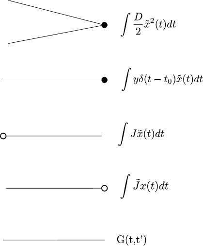
can be thought of in terms of these pairings. The idea is that with each $V_{mn}$ in $S_{I}$ we associate an internal vertex having $m$ entering edges and $n$ exiting edges. The $\int{J}\tilde{x}$ and $\int\tilde{J}{x}$ terms contribute, respectively, entering and exiting external vertices. Edges connecting vertices then correspond to a pairing between an $x(t)$ and $\tilde{x}(t)$. Finally, since

then only the terms in the expansion for $Z$ having $N$ entering and $M$ exiting external vertices (and thus $N$ and $M$ auxillary terms) will contribute to that moment. These terms are represented by *Feynman diagrams, *which is a graph composed of a combination of these vertices and in which each of the $N$ external vertices is connected (paired with) $M$ external vertices, possibly through a number of the internal vertices. Moments can be simply computed by writing down all possible diagrams with the requiste number of external vertices.

As an example, the coupling between external vertex $\int\tilde{J}x\, dt$ and internal vertex $\int\delta(t-t_{0})y\tilde{x}(t)\, dt$ in $Z$ can be evaluated as:

But this is best explained diagrammatically. In our case we have:

and the relevant vertices are illustrated in Figure 1. The process for then computing the first and second moment for the OU process is illustrated in Figure 2. We can see that each term will be written as an integral involving the auxillary functions $J$, $\tilde{J}$ and the propagator $G$. In general, each vertex in each diagram is assigned temporal index $t_{k}$.

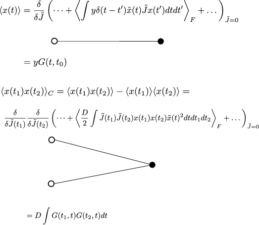
In OU, in fact only a finite number of diagrams can be considered and the exact mean and covariance can be determined. This is a result of the linearity of the SDE: a linear SDE can be written to have no $x$ terms in $S_{I}$, which means all internal vertices have no entering edges and that all moments in $x$ must correspond to a finite number of diagrams (in contrast to internal vertices with both entering and exiting edges which can then be combined in an infinite number of ways). In this case, from Figure 2, the mean and covariance are given by:

and

In summary, we’ve seen how to construct a path integral formulation of a generic SDE. And have seen how to construct Feynman diagrams perform perturbation expansions for the solution. In a follow-up post we will consider more examples of how they can be used.