In this follow-up post, we explore how some theory of convex functions and optimization relates to a common and powerful method in optimization – Lagrange multipliers

1. Conjugate functions

To being, we’ll introduce the concept of a conjugate function. Let \(f:\mathbb{R}^n\to\mathbb{R}\), then we can define \(f^*:\mathbb{R}^n\to\mathbb{R}\) as

\[f^*(\lambda) = \sup_{x\in\text{dom} f} (\lambda^T x - f(x)).\]

As you’ll recall from our last post, as this is the pointwise supremum over a set of convex (linear) functions, it is itself convex. This is true regardless of whether \(f\) is convex. This is known as the conjugate of \(f\).

How can this be convex even if \(f\) is not? Here’s one example:

Consider the non-convex function \(f(x) = x^2(x-1)(x+1)\)

Its conjugate is obtained through computing the following maximum:

Which is clearly convex.

Some more examples

1. Affine functions. If \(f(x) = ax+b\) then \(f^*:\{a\}\to\mathbb{R}$ and $f^*(a) = -b\)
2. Exponential. If \(f(x) = \exp(x)\) then \(f^*:\mathbb{R}_+\to\mathbb{R}\) and \(f^*(x) = x\log x - x\)
3. Negative entropy. If \(f(x) = x\log x\) then \(f^*(x) = \exp(x-1)\).
4. Strictly convex quadratic function. If \(f(x) = \frac{1}{2}x^TQx\) with \(Q\) positive definite, then \(f^*(x) = \frac{1}{2}x^TQ^{-1}x\)

If \(f(x)\) is convex then, given some additional technical condtions, \(f(x) = f^{**}(x)\), justifying the use of the term conjugate.

2. Lagrangian duality

The conjugate relates to an important concept in convex optimization, known as Lagrangian duality.

This can be thought of as a generalization of a common method in optimization, that of Lagrange multipliers, which I’ll review first.

2.1 Lagrange multipliers

Let’s consider the optimization problem

\[\min f(x)\\ h_i(x) = 0\]

Unlike above, here we don’t (yet) assume \(f(x)\) is convex.

Lagrange multipliers are a method for solving this constrained minimization problem by converting it into an unconstrained problem. This can be generalized (see below), but the basic method I’ll present in this section only deals with equality constraints.

The idea is to augment the objective function with a weighted sum of the constraint functions, forming what is known as the Lagrangian:

\[\mathcal{L}(x, \nu) = f(x) + \sum_{i=1}^p \nu_i h_i(x)\]

The variables \(\nu_i\) are known as the Lagrange multipliers.

The basic idea is that by looking for stationary points of the unconstrained Lagrangian

\[\nabla \mathcal{L}(x,\nu) = 0\]

we can obtain solutions to the original problem. Why does this work? First note that solving \(\frac{\partial \mathcal{L}}{\partial x} = 0\) and \(\frac{\partial \mathcal{L}}{\partial \nu}=0\) gives:

\[\begin{align*} \frac{\partial \mathcal{L}}{\partial x} = 0 &\Rightarrow \nabla_x f(x) + \sum_{i=1}^p \nu_i \nabla_x h_i(x) = 0\\ \frac{\partial \mathcal{L}}{\partial \nu} = 0 &\Rightarrow h_i(x) = 0, \forall i \end{align*}\]

Thus finding stationary points of \(\mathcal{L}\) will correspond to points satisfying the constraints.

But why should it minimize the function given the constraint? The graphical intuition is the following:

2.2 The dual problem

The dual function

Let’s begin the process of generalizing this approach to deal with inequality constraints, too. That is, let’s turn to the problem

\[\min f(x)\\ g_i(x) \le 0,\quad i = 1, \dots, m \\ h_j(x) = 0,\quad i = 1, \dots, p\]

Define the Lagrangian of the this problem as:

\[\mathcal{L}(x, \lambda, \nu) = f(x) + \sum_{i = 1}^m\lambda_i g_i(x) + \sum_{j=1}^p\nu_i h_i(x)\]

Again, \(\lambda\) and \(\nu\) are Lagrange multipliers, or dual variables.

From this we can define the Lagrange dual function:

\[g(\lambda, \nu) = \inf_{x\in\mathcal{X}}\mathcal{L}(x, \lambda, nu).\]

Now, we use the same property as above: the pointwise infimum (read minimum) of a family of affine functions of \((\lambda,\nu)\) is concave. This is true even when the optimization problem above is not convex.

For a common problem class there is a relation between the dual function and the conjugate that can facilitate computation of \(g(\lambda, \nu)\). For problems of the form:

\[\min f(x)\\ Ax \preceq b,\\ Cx = d\]

then

\[\begin{align} g(\lambda, \nu) &= \inf_x \left(f(x) + \lambda^T (Ax-b) + \nu^T(Cx-d) \right)\\ &= -b^T\lambda - d^T\nu + \inf_x \left(f(x) + \lambda^T (A^T\lambda + C^T\nu)x \right)\\ &= -b^T\lambda - d^T\nu -f^*(-A^T\lambda - C^T\nu) \end{align}\]

An important property is that the dual function is a lower bound for the solution to the original problem. Call \(p^*\) the minimum obtained at the optimal solution to the problem: \(p^* = f(x^*)\).

The original problem is known as the primal problem. Then, we have:

\[g(\lambda, \nu) \le p^*\]

for any \(\lambda \succeq 0\) and for any \(\nu\).

This is easy to show: the optimal \(x^*\) satisfies the constraints \(g_i(x)\le 0\) and \(h_i(x) = 0\), thus

\[\sum_{i=1}^m\lambda_ig_i(x^*) \le 0\]

and

\[\sum_{i=1}^p\nu_ih_i(x^*) = 0\]

thus

\[L(x^*, \lambda, \nu) = f(x^*) + \sum_{i=1}^m\lambda_ig_i(x^*) + \sum_{i=1}^p\lambda_ih_i(x^*) \le f(x^*).\]

This means:

\[g(\lambda, \nu) = \inf_x L(x, \lambda, \nu) \le L(x^*, \lambda, \nu) \le f(x^*) = p^*\]

The dual problem

Ok, so what do we do with this lower bound? A natural thing to do is to ask, how high can we make this lower bound? This is the dual problem:

\[\max_{\lambda \succeq 0, \nu} g(\lambda, \nu)\]

The solution is denoted \((\lambda^*, \nu^*)\), the dual optimal solution. Since this is a maximization of a concave function, it is a convex problem, even if the primal problem is not.

Call \(d^* = g(\lambda^*, \nu^*)\). Then, from above, we have

\[d^*\le p^*\]

The difference \(p^* - d^*\) is known as the optimal duality gap.

This general inequality is known as weak duality. Even weak duality can be useful. As in some cases the dual problem may be efficiently solvable (being a convex problem) while the original one is much more challenging. Thus it can be useful to find a lower bound on the primal solution.

Strong duality

When the gap is zero:

\[d^* = p^*\]

then strong duality holds. Now the dual problem can say a lot more about our original problem, which we’ll cover momentarily. Strong duality holds when the problem is convex: this is known as Slater’s condition. But it can hold under other conditions also.

Some examples

This has been quite a bit of theory. So what are some examples of these concepts?

Well, let’s consider again the simple quadratic function \(f(x) = x^2/2\) with inequality constraints \(x - a \le 0\). The Lagrangian is

\[L(x, \lambda) = x^2/2 + \lambda(x-a)\]

thus the dual function is

\[g(\lambda) = \inf_x L(x, \lambda) = -\lambda^2/2 - \lambda a\]

We can see that by maximizing \(g(\lambda)\) over \(\lambda \ge 0\) we get:

\[\lambda^* = \max(-a, 0), \quad d^* = \begin{cases} a^2/2, \quad a < 0;\\ 0, \quad a \ge 0 \end{cases}\]

which matches the optimal solution \(p^*\).

Strong duality holds here, as we can see in this olot. The top axes show the original optimization problem, with the red line indicating the primal optimal solution. The bottom axes show the dual optimization problem, with the dashed line showing the dual optimal solution. We can see the red and dashed lines overlap, regardless of the value of \(a\).

What if we try with a non-convex function? Now let \(f(x) = -x^3+x\), again with \(x\le a\).

This time we do have a duality gap, as evidenced by the gap between the red and dashed curves.

Min-max interpretation

As in interesting aside, the primal problem can be expressed in a way that gives a nice symmetry to the two problems.

Consider the case where we only have inequality constraints. Then we have:

\[\sup_{\lambda \succeq 0} L(x,\lambda) = \sup_{\lambda \succeq 0}\left(f(x) + \sum_{i=1}^m \lambda_i g_i(x)\right) = f(x)\]

This is because, provided the constraints are satisfied, \(g_i(x) \le 0\) and the best choice is \(\lambda = 0\). Thus we can write:

\[p^* = \inf_x f(x) = \inf_x \sup_{\lambda \succeq 0} L(x,\lambda)\]

and, by our earlier definitions, we have:

\[d^* = \sup_{\lambda\succeq 0}\inf_x L(x,\lambda).\]

This means weak duality implies:

\[\sup_{\lambda\succeq 0}\inf_x L(x,\lambda) \le \inf_x \sup_{\lambda\succeq 0} L(x,\lambda).\]

This is in fact a general result that any function \(f(x,\lambda)\) satisfies. This is known as the max-min inequality.

Strong duality implies:

\[\sup_{\lambda\succeq 0}\inf_x L(x,\lambda) = \inf_x \sup_{\lambda\succeq 0} L(x,\lambda)\]

(This is also known as the saddle point property, because the optimal point \((x^*, \lambda^*)\) is in fact a saddle point of \(L\). This result is known as the minimax theorem, proved by von Neumann in the context of his work on game theory).

We can see the saddle point property at play if we plot the Lagrangian for our earlier quadratic problem:

\[\min x^2, \quad x \le a\]

The Lagrangian is:

\[L(x, \lambda) = x^2 + \lambda(x-a)\]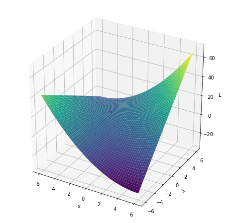

3. Generalizing Lagrange multipliers: the KKT conditions

Complementary slackness

When strong duality holds we have an important property of the optimal solution known as complementary slackness.

We have

\[\begin{align} f(x^*) &= g(\lambda^*, \nu^*)\\ &= \inf_x\left(f(x) + \sum_{i=1}^m\lambda^*_i g_i(x) + \sum_{i=1}^p\nu^*_i h_i(x)\right)\\ &\le f(x^*) + \sum_{i=1}^m\lambda^*_i g_i(x^*) + \sum_{i=1}^p\nu^*_i h_i(x^*)\\ &\le f(x^*) \end{align}\]

This implies that

\[\sum_{i=1}^m \lambda_i^* g_i(x^*) = 0\]

and, since each term in the sum is nonpositive, then in fact each term must be zero:

\[\lambda_i^* g_i(x^*) = 0, \quad i = 1, \dots, m.\]

Usefully, this property gives additional equality constraints a solution must satisfy to be optimal. In particular, it means that either \(\lambda_i^* = 0\) or \(g_i(x^*) = 0\). In other words, when \(\lambda_i^* > 0\) then the inequality constraint \(g_i\) must be tight. If \(\lambda_i = 0\) then it can be slack.

We actually saw complementary slackness at play in our simple quadratic example above. If we plot \(g(x^*) = x^* - a, \lambda^*\) as a function of the inequality constraint parameter \(a\) (recall \(x \le a\)):

We see for \(a\le 0\) the constraint is tight, and \(x^* = a\). For \(a>0\), then the optimal solution is \(x^* = 0\), and \(x^* - a\) becomes slack.

KKT for non-convex problems

Here we assume the functions \(f(x), g_i(x), h_i(x)\) are all differentiable. We can argue that \(x^*\) minimizes \(L(x, \lambda^*, \nu^*)\), and therefore the gradient must vanish at \(x^*\):

\[\nabla f(x^*) + \sum_{i=1}^m\lambda_i^*\nabla g_i(x^*) + \sum_{i=1}^p\nu_i^*\nabla h_i(x^*) = 0\]

Now we’re in a position to see how all this theory relates to our optimization problem, when strong duality obtains.

Let’s collect conditions an optimal solution \((x^*, \lambda^*, \nu^*)\) must satisfy, for problems with strong duality. We have:

\[\begin{align} g_i(x^*) &\le 0, \quad i=1, \dots, m\\ h_i(x^*) &= 0, \quad i=1, \dots, p\\ \lambda^*_i &\ge 0, \quad i=1, \dots, m\\ \lambda_i^* g_i(x^*) &= 0, \quad i=1, \dots, m\\ \nabla f(x^*) + \sum_{i=1}^m\lambda_i^*\nabla g_i(x^*) + \sum_{i=1}^p\nu_i^*\nabla h_i(x^*) &= 0 \end{align}\]

These are known as the Karush-Kuhn-Tucker (KKT) conditions. They are necessary conditions for an optimal solution.

Note that if we have no inequality constraints, the above conditions simplify to the method of Lagrange multipliers that we discussed above:

\[\begin{align} h_i(x^*) &= 0,\quad i =1, \dots, p\\ \nabla f(x^*) + \sum_{i=1}^p\nu_i^*\nabla h_i(x^*) &= 0 \end{align}\]

KKT for convex problems

When the primal problem is convex, the KKT conditions are also sufficient for an optimal solution.

To summarize all of the above: for any differentiable optimization problem for which strong duality obtains, the KKT conditions provide necessary conditions for an optimal solution. Algorithms focus on finding all points which satisfy such conditions, and from those finding the globally optimal solution.

When the problem is convex, KKT is also sufficient, and any solution that satisifes the conditions is optimal.

Outside of convexity, there are a range of other constraint qualifications that imply that a particular problem has strong duality, and therefore that KKT is relevant.

Take-home messages

After going through this tutorial, you should now know:

• What convexity is and why it is important for optimization
• How some properties of convex functions are used to prove convergence of gradient descent
• What primal and dual optimization problems are
• How the KKT conditions generalize Lagrange multipliers for inequality constraint problems