Here I cover a basic introduction to concepts and theory of convex optimization. The goal is to give an impression of why this is an important area of optimization, what its applications are, and some intiution for how it works. This is of course not meant to overview all areas of convex optimization, it’s a huge topic, but more to give a flavor of the area by describing some results and theory, particularly as they relate to other areas that may be familiar to some (e.g. the method of Lagrange multipliers). By presenting this in a notebook the aim is to focus on providing some geometric intuition whenever possible through plotting simple examples whose parameters you can play with. Images not generated in this notebook are taken from one of the standard references: Convex Optimization, by Boyd and Vandenberghe.

This will be a (for the moment) two part post. In this part I will cover:

1. Why care about convexity?
2. Basics of convex functions and sets
3. A convergence proof of gradient descent

It will assume some basic familiarity with the idea of optimization, linear algebra and some machine learning basics.

Overview

Most machine learning problems end up as some form of optimization problem, thus a basic understanding of optimization is very useful, or sometimes necessary, to solve a given problem.

For instance, in simple linear regression, given some data \((y, X)\) and a model \(y \sim X\beta + \epsilon\), we aim to find the weights \(\beta\) that minimize:

\[\beta^* = \text{argmin}_\beta \|y - X\beta\|^2_2.\]

In general, we consider the following basic problem:

\[x^* = \text{argmin}_{x\in\mathcal{X}} f(x)\]

subject to constraints:

\[g_i(x) \le 0\\ h_j(x) = 0.\]

Convex optimization deals with problems in which \(f(x)\) and \(g_i(x)\) are convex functions, and \(h_j(x)\) are affine (of the form \(a_j^Tx = b_j\)).

1. Why care about convex optimization?

There are a range of reasons:

1. When your problem is convex, a locally optimal solution is globally optimal -> Can use gradient-based methods confidently
2. Shows up in common optimization problems
   • Linear least squares
   • Logistic regression
   • Weighted least squares
   • Any of these with L1 or L2 regularization
3. There is a lot of associated theory. Convexity is quite a strict requirement, this provides a lot of structure, which mean we can apply strong theory and geometric intuitions which can provide a good understanding of a problem
4. Can be relevant even for non-convex problems:
   • Can turn into a convex problem (primal -> dual problem, see below)
   • Can approximate with a convex function to initialize a local optimization method
   • Common heuristics: convex relaxation for finding sparse solutions, e.g. \(L_0\) to \(L_1\) relaxation
   • Bounds for global optimization
5. Concepts that naturally arise in convex optimization are important elsewhere, like the theory of Lagrangians

Somewhat like linear algebra, because you can do a lot with convex optimization, it is quite foundational to optimization.

Ok, but what is a convex function?

2. Basics of convex functions and sets

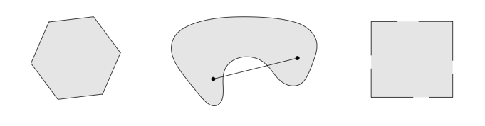
A convex set is a set \(C\) in which the line segment connecting any two points in the set is also in the set. That is, if \(x_1,x_2\in C\) and \(0\le \theta \le t\) then

\[\theta x_1 + (1-\theta)x_2 \in C.\]

Some examples (the middle one is not convex):

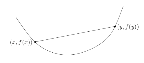
A function \(f:\mathbb{R}^n\to\mathbb{R}\) is convex if \(\text{dom} f\) is convex and for \(0\le \theta \le 1, x_1, x_2 \in \text{dom} f\):

\[f(\theta x_1 + (1-\theta)x_2) \le \theta f(x_1) + (1-\theta) f(x_2)\]

This means that a line segement connecting any two points in the domain of \(f\) lies above the graph of \(f\):

An alternative definition

If \(f\) is differentiable, then \(f\) is convex if and only if \(\text{dom} f\) is convex and

\[f(y) \ge f(x) + \nabla f(x)^T(y-x)\]

holds for all \(x,y\in\text{dom} f\).

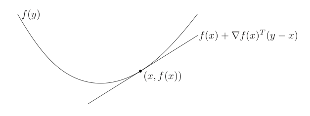
This means local information of a convex function can tell us about global information of the function – this is a key property of convex functions.

For instance, if \(\nabla f(x) = 0\) then for all \(y\in\text{dom} f\) it is the case that \(f(y) \ge f(x)\). In other words, \(x\) is a global minimizer of \(f\).

A few more definitions:

Strict convexity

A function \(f\) is strictly convex if the inequality holds whenever \(x\ne y\). I.e. a linear function is not strictly convex

Strong convexity

Strong convexity implies there is some positive \(m\) such that:

\[\nabla^2 f(x) \succeq mI\]

which can be shown to be equivalent to

\[f(y) \ge f(x) + \nabla f(x)^T(y-x) + \frac{m}{2}\|x - y\|^2_2\]

for all \(x,y\in \mathcal{X}\).

This means the function can be lower bounded by a quadratic function with some fixed second derivative \(mI\) at all points \(x\in\mathcal{X}\).

Some examples of convex functions

1. The indicator function of a convex set, \(S\).

If \(I_S(x)\) is defined as

\[I_S(x) = \begin{cases} 0, \quad x\in S;\\ +\infty, \quad\text{else} \end{cases}\]

Then \(I_S(x)\) is convex

1. Norms. Any norm is a convex function. Here is the \(L_1\) norm:

1. Quadratic functions: \(f(x) = x^T P x + 2q^T x + r\) for \(P\) positive definite. The linear least squares in the introduction is a quadratic function of this form. For example:

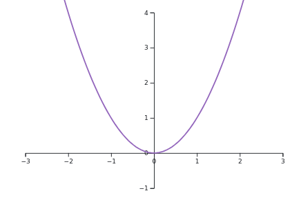
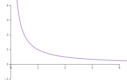
1. Common functions: \(1/x\) for \(x>0\), \(e^x\) for \(x\in\mathbb{R}\), \(x^2\) for \(x\in\mathbb{R}\). For instance:

Examples of strong convexity

\(f(x) = x^2\), somewhat trivally, is a strongly convex function.

\(f(x) = \exp(x)\) is not a strongly convex function. The general idea being something like functions that become arbitarily flat/linear in some direction are not strongly convex. This is simply shown below, in which for the quadratic function, we can find an \(m\) such that a quadatic approximation at any point \(x_0\) with second derivative \(m\) is always below \(f(x)\). This is not true for the exponential function.

Operations that preserve convexity

Convexity is a strong property. So it’s good to know when we can preserve it.

1. Non-negative weighted sums.

If \(f_i\) are each convex, then the nonnegative weighted sum:

\[f(x) = \sum_i w_i f_i(x)\]

is convex, for \(w_i \ge 0\).

1. Composition with nondecreasing functions.

Let \(f = h(g(x))\). If \(h\) is a scalar function, \(h:\mathbb{R}\to\mathbb{R}\), then:

For example, if \(h\) is convex and nondecreasing, and \(g\) is convex, then \(f\) is convex.

1. Pointwise maxima.

If \(f_1\) and \(f_2\) are convex, then the pointwise maximum:

\[f(x) = \max\{f_1(x), f_2(x)\}\]

is also convex. The proof is simple:

\[\begin{align} f(\theta x + (1-\theta)y) &= \max\{f_1(\theta x + (1-\theta)y), f_2(\theta x + (1-\theta)y)\}\\ &\le \max\{\theta f_1(x) + (1-\theta)f_1(y), \theta f_2(x) + (1-\theta)f_2(y)\}\quad\text{(conv. of $f_1,f_2$)}\\ &\le \theta\max\{ f_1(x), f_2(x) \} + (1-\theta)\max\{f_1(y),f_2(y)\}\quad\text{(replace $f_1$ w. max $f_1,f_2$)}\\ &= \theta f(x) + (1-\theta) f(y) \end{align}\]

This result extends to pointwise maximum over \(n\) functions:

\[f(x) = \max\{(f_i(x)\}_{i=1}^n\]

and also the pointwise supremum over an infinite set of convex functions. Let \(\{f_i(x)\}_{i\in I}\) be a collection of convex functions, then

\[g(x) = \sup_{i\in I}f_i(x)\]

is convex.

3. Convergence of gradient descent

We demonstrate how the ideas presented here can be used to study optimization algorithms. We’ll prove the convergence of gradient descent for strongly convex functions. The argument is as follows.

For a strongly convex function that satisfies:

\[\alpha I \preceq \nabla^2 f(x) \preceq \beta I\]

for all \(x\in\mathcal{X}\) and \(0<\alpha \le \beta\), an equivalent condition is for

\[f(y) \ge f(x) + \nabla f(x)(y-x) + \frac{\alpha}{2}\|y-x\|^2,\quad \forall x,y\in\mathcal{X}\]

known as \(\alpha\)-strongly convex. And the relation condition

\[f(y) \le f(x) + \nabla f(x)(y-x) + \frac{\beta}{2}\|y-x\|^2,\quad \forall x,y\in\mathcal{X}\]

is known as \(\beta\)-smoothness.

In other words, for all points \(x\in\mathcal{X}\), the function \(f(y)\) can be bounded below and above by quadratic functions intersecting at \(f(x)\).

This can be used to show the following inequalities:

\[\begin{align} \frac{\alpha}{2}\|x^* - x\|^2&\le f(x) - f(x^*) \le \frac{1}{2\alpha}\|\nabla f(x)\|^2\quad \text{$\alpha$-strongly convex}\\ \frac{\beta}{2}\|x^* - x\|^2&\ge f(x) - f(x^*) \ge \frac{1}{2\beta}\|\nabla f(x)\|^2\quad\text{$\beta$-smoothness}\\ \end{align}\]

Call the quantity \(h(x) = f(x)-f(x^*)\) the primal gap, the thing we are trying to reduce in our optimization.

These inequalities are useful because they let us bound the primal gap by the gradient and the amount we’re moving in \(x\) (a property of the algorithm, which is known).

Now consider the gradient descent update:

\[x_{t+1} = x_t - \frac{1}{\beta}\nabla f(x_t)\]

Then the above inequalities can be used to show how the primal gap converges:

\[\begin{align} h_{t+1} - h_t &= f(x_{t+1}) - f(x_t)\\ &\le \nabla f(x_t)(x_{t+1}-x_t) + \frac{\beta}{2}\|x_{t+1}-x_t\|^2\quad (\text{$\beta$-smoothness})\\ &= -\frac{1}{\beta}\|\nabla f(x_t)\|^2 + \frac{1}{2\beta}\|\nabla f(x_t)\|^2\quad (\text{definition of algorithm})\\ &= -\frac{1}{2\beta}\|\nabla f(x_t)\|^2\quad\\ &\le -\frac{\alpha}{\beta}h_t\quad\\ \end{align}\]

Thus

\[h_{t+1} = h_t(1 - \frac{\alpha}{\beta}),\]

or

\[h_{t} = h_0(1 - \frac{\alpha}{\beta})^t.\]

Since \(\alpha < \beta\) then the algorithm converges. Further, how close \(\alpha\) is to \(\beta\) determines the convergence rate – convergence is fastest when \(\alpha\) is close to \(\beta\). This corresponds to the Hessian being closed to spherical (well-conditioned).

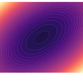
As an example, consider the quadratic function:

\[f(x,y) = \frac{m_x}{2}x^2 + \frac{m_y}{2}y^2.\]

This is strongly convex, with \(\alpha = \min(m_x, m_y)\) and \(\beta = \max(m_x, m_y)\). In the below widget we observe the convergence behavior (the primal gap as a function of gradient descent iteration). The green trace in the widget below shows the progression of the optimization for 20 iterations, after starting at (1,1). You can play with the functions parameters to see how that affects the rate of convergence. Apart from the first iteration, it’s linear on a log scale, as the above analysis would suggest. The slope depends on the ratio between \(\alpha\) and \(\beta\).

Conclusion

We’ve seen here the basic components of convex optimization, including what convexity is, some properties of convex functions, and how these relate to optimization with gradient descent. In the next post we will study how the theory of convex functions applies to Lagrange optimization and related concepts.